CMA-ES (Covariance Matrix Adaptation Evolution Strategy) in MATLAB

Background: evolution strategies

Evolution Strategy (ES) is one of the earliest evolutionary algorithms. It was developed by Ingo Rechenberg and Hans-Paul Schwefel in the 1960s, at about the same time as evolutionary programming and genetic algorithms. ES is based on adaptation and evolution, and its main idea is the evolution of evolution: the parameters that control the search, such as the step size, adapt during the run. ES is a family of related algorithms, so the plural name Evolution Strategies is also widely used. For more detail, see this article (opens in a new tab) on Wikipedia.

CMA-ES

The Covariance Matrix Adaptation Evolution Strategy (CMA-ES) adapts a multivariate Gaussian search distribution. It was proposed by Nikolaus Hansen and Andreas Ostermeier in 2001, in this paper (opens in a new tab). The paper describes completely derandomized self-adaptation in evolution strategies.

CMA-ES builds a Gaussian probabilistic model of promising solutions and uses this model to create the next generation. This makes CMA-ES an Estimation of Distribution Algorithm (EDA). For more on EDAs, see the Wikipedia article (opens in a new tab).

How CMA-ES works

The search distribution is a multivariate normal distribution with a mean $m$, a global step size $\sigma$ and a covariance matrix $C$. Each generation has four steps.

1. Sampling. Create $\lambda$ new solutions:

2. Updating the mean. Sort the samples by cost and move the mean toward a weighted average of the best $\mu$ of them:

where $y_{j:\lambda}$ is the step of the $j$th best sample. The weights decrease with rank, $w_j \propto \ln(\mu + 0.5) - \ln j$, and sum to 1.

3. Adapting the step size. An evolution path $p_\sigma$ adds up the recent steps of the mean. If the steps point in the same direction again and again, the path becomes long and $\sigma$ grows. If they cancel each other out, the path is short and $\sigma$ shrinks. The length of $p_\sigma$ is compared with its expected length under random selection, $E\lVert\mathcal{N}(0, I)\rVert$.

4. Adapting the covariance matrix. $C$ is updated from two sources: a rank one update from a second evolution path $p_c$, and a rank $\mu$ update from the steps of the $\mu$ best samples:

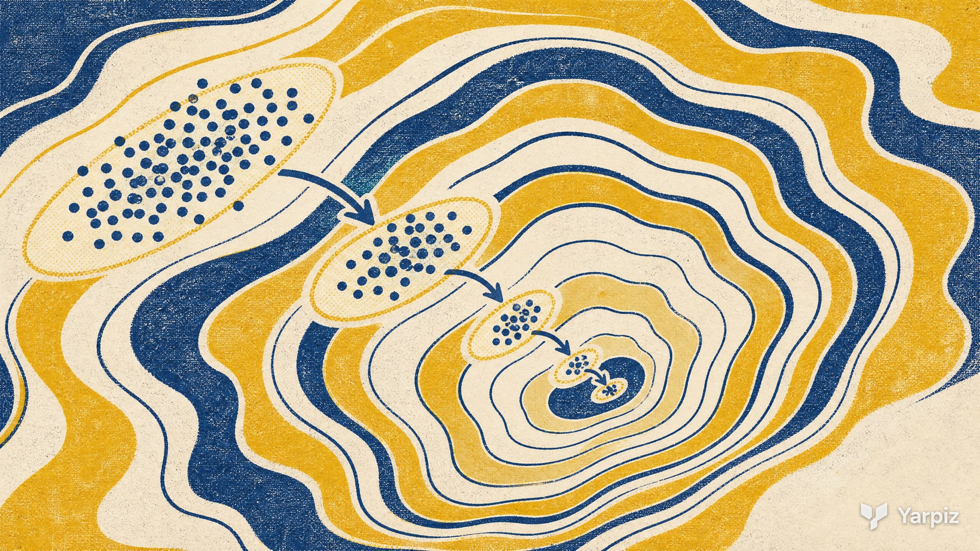
Over time, $C$ learns the shape of the cost function near the current mean. On a long, narrow valley, for example, the distribution stretches along the valley. This is why CMA-ES handles badly scaled and correlated variables well.

MATLAB implementation

This post shares a structured open-source implementation of CMA-ES in MATLAB. If you know MATLAB, you should find it easy to use the code in your research and projects.

The CMA-ES folder holds the algorithm in cmaes.m, a one line entry point main.m, and four test functions: Sphere.m, Ackley.m, Rastrigin.m and Rosenbrock.m. The default cost function is Ackley. To run the code, open the folder in MATLAB and run main.m. The program prints the best cost in every iteration and plots the best cost against the iteration on a logarithmic scale.

The script samples with mvnrnd and creates the first mean with unifrnd. Both are functions of the Statistics and Machine Learning Toolbox, so the code probably needs that toolbox.

Parameters in the code

The problem and the main settings are at the top of cmaes.m:

The value of lambda is ten times the usual default population size of about $4 + 3 \ln n$. The learning rates (cs, ds, cc, c1 and cmu) are computed in the script from $n$ and from the effective number of parents $\mu_{\text{eff}} = 1/\sum_j w_j^2$. Samples and the new mean are clipped to the variable bounds.

To solve your own problem, write a cost function that takes a row vector and returns a number, and set CostFunction, nVar, VarMin and VarMax at the top of cmaes.m.

Check the result

Begin with the default Ackley function and compare repeated runs before changing the objective. Inspect the best cost, the final coordinates, and the evaluation budget, since each generation samples many candidates. The implementation clips samples at the bounds, so a boundary-heavy problem can behave differently from an unconstrained Gaussian search. Increasing lambda also increases the work per generation and should be considered when comparing iteration counts.

Related posts

• The YPEA toolbox, Yarpiz Evolutionary Algorithms, also includes CMA-ES with a common problem definition.

Mostapha Kalami Heris, CMA-ES (Covariance Matrix Adaptation Evolution Strategy) in MATLAB (YPEA108), Yarpiz, 2015. https://yarpiz.com/cma-es-ypea108

@misc{yarpiz-ypea108,
  author = {{Mostapha Kalami Heris}},
  title = {{CMA-ES (Covariance Matrix Adaptation Evolution Strategy) in MATLAB}},
  howpublished = {Yarpiz},
  year = {2015},
  note = {Code YPEA108},
  url = {https://yarpiz.com/cma-es-ypea108}
}