Principal Component Analysis (PCA) in Python and MATLAB: Free Video Course

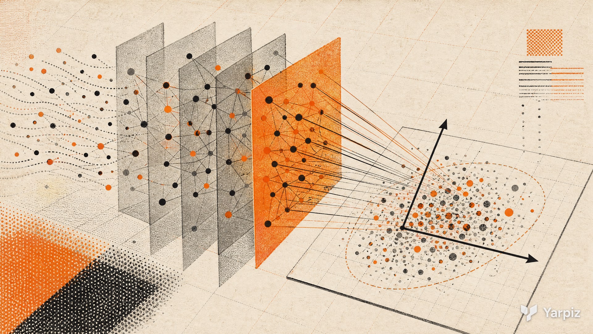
Principal Component Analysis (PCA) is a statistical procedure and an unsupervised learning algorithm for reducing the dimensionality of a data set while retaining as much variance as possible for the chosen number of components. It finds a set of new variables, called principal components, that are linear combinations of the original variables. The components are uncorrelated with each other, and they explain as much of the variance in the data as possible.

This free video course explains the idea and the mathematics of PCA, and then implements it step by step, first in Python and then in MATLAB. The video is about 1 hour 20 minutes long. The course is taught by Mostapha Kalami Heris.

The idea behind PCA

PCA is a linear transformation. It maps data from a $d$ dimensional space to a space with the same number of dimensions, with orthogonal axes and uncorrelated component scores after centering. Keeping only the first few of them reduces the number of dimensions.

The video starts with a simple question. Assume each sample has two features $x$ and $y$, for example the blood pressure and the heart rate of a patient, or the return and the risk of a stock. If only one feature may be kept, the wise choice is the one with the larger variance, because it carries more of the spread in the data. But a new variable $z = c_1 x + c_2 y$, a linear combination of both, can have an even larger variance. Keeping $x$ alone ($c_1 = 1$, $c_2 = 0$) or $y$ alone is only a special case. PCA answers the question: which coefficients give the largest possible variance?

The mathematics

Let each sample be a vector $x_i \in \mathbb{R}^d$, for $i = 1, \dots, n$, with the sample mean $\bar{x}$ and the covariance matrix

$C$ is a symmetric $d \times d$ matrix, and its eigenvalues are non-negative. For a coefficient vector $u$, the new variable is $z = u^T x$, and its variance simplifies to

This value grows without limit when $u$ grows, so the search is limited to unit vectors, $u^T u = 1$. With a Lagrange multiplier $\lambda$, the problem becomes the maximization of

Setting the derivative with respect to $u$ to zero gives

So $u$ must be an eigenvector of the covariance matrix, and $\lambda$ is its eigenvalue. Putting this back into the objective gives $\operatorname{Var}(z) = u^T \lambda u = \lambda$. The variance of $z$ equals the eigenvalue, so the best direction is the eigenvector of the largest eigenvalue. This is the first principal component.

To map the data to $m$ dimensions, the transformation uses a $d \times m$ matrix $U = [u_1, u_2, \dots, u_m]$ and centered scores $z = U^T(x - \bar{x})$. Its columns are the eigenvectors of $C$ sorted by their eigenvalues in descending order, $\lambda_1 \ge \lambda_2 \ge \dots \ge \lambda_d$. The components of $z$ then have the largest possible variances, and they are uncorrelated.

A transformed sample can be mapped back to the original space with $\hat{x} = \bar{x} + U z$. This gives the projection of the sample onto the principal components. Because no labels or target values are used anywhere, PCA is an unsupervised method.

Explained variance

The share of the total variance kept by the first $m$ components is

Plotting this ratio against $m$ shows how many components retain a chosen share of variance. That share is not the same as predictive information about a target.

What the video covers

Theory (from 00:06)

The two feature example, the linear combination $z = u^T x$, the covariance matrix, the variance $u^T C u$, the unit length constraint, the Lagrange multiplier, and the eigenvalue solution. The video then extends the result from one component to $m$ components.

Python from scratch (from 24:19)

A Jupyter notebook implements PCA with NumPy only, without any PCA library. It creates 1,000 samples of two independent standard normal variables with a seeded generator (np.random.RandomState(0)). The cloud of points is round, so every direction has a similar variance. Multiplying the data by a random $2 \times 2$ matrix makes the cloud stretched and correlated, like real data.

The notebook then computes the covariance matrix with np.cov(X.T) and its eigenvalues and eigenvectors with np.linalg.eig. It picks the eigenvector of the largest eigenvalue and computes $z$ with np.dot. The variance of $z$ is larger than the variance of either original feature, and it is close to the largest eigenvalue. Finally, np.outer maps $z$ back to two dimensions, and the plot shows the projected points on a line along the first principal component. The second eigenvector gives the perpendicular direction.

PCA with scikit-learn (from 38:13)

The second notebook uses the PCA class from sklearn.decomposition and the data sets in sklearn.datasets.

• Iris data set. 150 flowers of three species, each described by four measurements (the length and width of the petal and the sepal). PCA(n_components=2), fit and transform reduce the four features to two. The components_ attribute holds the eigenvectors. In the scatter plot of the two components, colored by species, one species is fully separated from the other two, and the other two are still largely separable.
• Handwritten digits (from 44:48). 1,797 images of $8 \times 8$ pixels. Each image is stored as a row of 64 pixel values, so every sample has 64 features. PCA reduces these 64 features to two components. In the plot, visually similar digits lie close together, for example 1 and 7, or 5 and 9, while 0 is almost separated from the others. The video notes that four or five components would retain more variance. Whether those features improve classification still needs a separate evaluation.

MATLAB from scratch (from 51:29)

The same steps are repeated in MATLAB with randn, rand, cov and eig. The script pca1.m finds the largest eigenvalue with max(diag(E)), takes the matching eigenvector, transforms the data with z = X*u, maps it back with z*u', and plots the data and its projection together.

MATLAB with the Statistics and Machine Learning Toolbox (from 64:49)

The script pca2.m loads the iris data with iris_dataset, transposes it so that each row is one sample, and converts the class labels with vec2ind. Then [U, Z] = pca(X, 'NumComponents', 2) returns the transformation matrix and the transformed data (the scores), and a colored scatter plot shows the two components.

The script pca3.m (from 71:13) reads the digits data from digits.csv with csvread. The first 64 columns are the pixel values and the last column is the digit. The video shows a few digits as images with imshow and plots the first two principal components. The script in the download keeps five components.

Explained variance (from 77:20)

At the end, the video sorts the eigenvalues of the digits covariance matrix in descending order and plots their cumulative sum divided by the total. The curve shows how cumulative explained variance grows with the number of components. The video estimates that about 13 components keep roughly 80 percent and about 30 components keep about 95 percent of the variance.

Check the result

Center data using the training mean and use that same mean when projecting new samples. Decide whether feature scaling is needed, since PCA follows variance and therefore depends on units. The covariance formula above uses $1/n$, while cov and np.cov commonly use $1/(n-1)$ in these examples. Keep the normalization consistent when comparing eigenvalues and variance. Fit PCA on training data only, and choose the component count using the intended reconstruction or prediction task rather than a two-dimensional plot alone.

Applications

PCA is used for dimensionality reduction, feature extraction, lossy data compression and the visualization of high dimensional data. A common use is preprocessing: fewer, uncorrelated features make classification, regression and other analyses easier and faster, as the digits example shows.

Files and requirements

The download has the two Python notebooks (PCA.ipynb and PCA using Scikit-Learn.ipynb) and the MATLAB scripts pca1.m, pca2.m and pca3.m with digits.csv.

• No specific data science experience is needed, but basic knowledge of data preparation and preprocessing helps.
• Python with NumPy, Matplotlib and scikit-learn, and MATLAB with the Statistics and Machine Learning Toolbox. The iris example in pca2.m probably also needs the Deep Learning Toolbox, which provides iris_dataset and vec2ind.

Related posts

• Linear Discriminant Analysis (LDA) in MATLAB, a supervised method for linear feature extraction.

Watch online

The video is available on the Yarpiz YouTube channel.

Play videoLoads from YouTube

Mostapha Kalami Heris, Principal Component Analysis (PCA) in Python and MATLAB: Free Video Course (YPPCA191211), Yarpiz, 2019. https://yarpiz.com/principal-component-analysis-in-python-and-matlab-video-tutorial-yppca191211

@misc{yarpiz-yppca191211,
  author = {{Mostapha Kalami Heris}},
  title = {{Principal Component Analysis (PCA) in Python and MATLAB: Free Video Course}},
  howpublished = {Yarpiz},
  year = {2019},
  note = {Code YPPCA191211},
  url = {https://yarpiz.com/principal-component-analysis-in-python-and-matlab-video-tutorial-yppca191211}
}