Linear Programming in MATLAB: Video Tutorial

Linear programming (LP) models decisions with a linear objective and linear constraints. This free video tutorial explains the model, solves an example with MATLAB’s linprog function and builds a transportation model from shipping costs, capacities and demands. Mostapha Kalami Heris teaches the 43 minute 5 second video.

What is linear programming?

Linear programming finds the best use of limited resources, such as time, money or materials. The goal is to maximize a profit or minimize a cost, and the problem is described with equations and inequalities. The values to choose, for example how many products to make, are the decision variables.

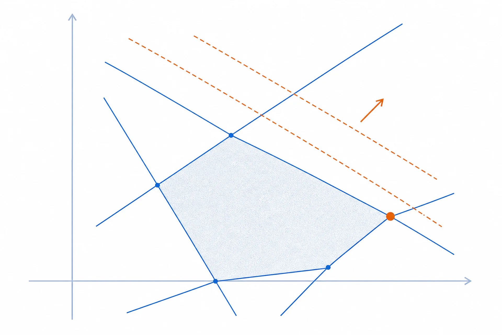
The conceptual sketch shows a two-variable feasible region and the direction in which an objective improves. It is not a plot of the numerical example below.

In an LP model, the objective function and every constraint are linear combinations of the decision variables. A small example from the video has three variables: maximize $x_1 + 2x_2 - x_3$, subject to constraints such as $x_1 + x_2 \le 5$ and $x_1 - 2x_2 + 3x_3 \le 10$. A model may also have equality constraints, such as a fixed value for $x_1 + x_3$.

The linear structure makes large continuous models practical to solve with established algorithms, including simplex and interior-point methods. A model can still be infeasible, unbounded or numerically difficult. LP is widely used in economics, engineering, logistics, supply chain management, production scheduling and financial portfolio optimization.

The general form

The video writes every LP problem in one matrix form:

Here $x$ is the vector of decision variables and $f$ holds the coefficients of the objective. Each row of $A$ and $b$ is one inequality constraint, each row of $A_{eq}$ and $b_{eq}$ is one equality constraint, and $lb$ and $ub$ are lower and upper bounds on the variables.

MATLAB solves this form with linprog, which is part of the Optimization Toolbox:

[x, fval] = linprog(f, A, b, Aeq, beq, lb, ub)

Two details matter when a problem is converted to this form:

• linprog always minimizes. To maximize $f^T x$, pass $-f$ and change the sign of the returned objective value.
• Every inequality must have the form “less than or equal to”. A constraint with $\ge$ is multiplied by $-1$.

Missing parts are passed as empty matrices [], for example when a problem has no equality constraints or no upper bounds.

A first example in MATLAB

The video solves this problem (from 04:08):

The second constraint is rewritten as $-x_1 + x_2 \le -3$. So $f = (5, 6)$, the rows of $A$ are $(1, 1)$, $(-1, 1)$ and $(5, 4)$, $b = (10, -3, 35)$, and $lb = (0, 0)$. There are no equality constraints and no upper bounds. The call uses $-f$ because the problem is a maximization. The solution is $x_1 \approx 5.222$ and $x_2 \approx 2.222$, with an objective value of about $39.444$. The video then collects these definitions into a script.

The transportation problem

The second half of the video (from 13:44) builds a classic LP model. A set of providers (factories or warehouses) ships a product to a set of consumers (customers). The example has two providers and three consumers, so it has six decision variables:

• $x_{ij}$ is the amount shipped from provider $i$ to consumer $j$.
• $c_{ij}$ is the cost of shipping one unit on that route.
• $s_i$ is the production capacity of provider $i$. In the example, the capacities are 900 and 800.
• $d_j$ is the demand of consumer $j$. In the example, the demands are 500, 600 and 300.

The model minimizes the total transportation cost while it respects the capacities and meets the demands:

Building the matrices with a function

Writing these matrices by hand does not scale to larger problems, so the video writes a MATLAB function that builds them from three inputs: the cost matrix, the vector of capacities and the vector of demands (from 19:12). The main steps are:

1. The number of providers and consumers comes from the size of the cost matrix.
2. The cost matrix is flattened into the vector $f$. MATLAB flattens a matrix column by column, so the variables are ordered $x_{11}, x_{21}, x_{12}, x_{22}, x_{13}, x_{23}$.
3. The function sub2ind finds the position of each $x_{ij}$ in this vector. A short anonymous function wraps it for convenience.
4. Each provider adds one row to $A$, with ones at the positions of its variables, and its capacity to $b$.
5. Each consumer adds one row as well. Because the demand constraints use $\ge$, these rows are $-1$ and the right side is $-d_j$.
6. The lower bounds are a vector of zeros. $A$ and $b$ are created with zeros in advance, because growing them inside the loop is slow for large problems.

The function returns all of this in one structure, which is passed to linprog. Finally, reshape turns the solution vector back into a matrix with one row per provider and one column per consumer.

Reading the solution

In the video’s example, the first provider supplies all of the second consumer’s demand, the second provider supplies all of the third consumer’s demand, and the two providers share the first consumer. Summing the solution matrix confirms that every demand is met. The first provider uses its full capacity of 900, while the second provider ships only 500 of its 800, because its routes cost more on average. When one of its costs is lowered, the solution changes and the second provider is used fully.

The same pattern works for other LP models: write a function that builds the matrices, pass them to linprog, and reshape the solution into the form the problem needs.

Check the model and result

Inspect the solver’s termination information, then verify the inequalities, equalities and bounds using the returned decision variables. A solver can accurately solve the wrong model if a sign, unit or variable order is incorrect. In the transportation example, check that row totals stay within supply and column totals meet demand. The model treats shipment amounts as continuous. Whole-unit decisions require an integer model rather than rounding the result afterward.

Who this tutorial is for

• Applied mathematics and engineering students
• Operations research (OR) students
• Anyone interested in mathematical optimization

It helps to know basic matrix and vector notation and to have MATLAB with the Optimization Toolbox, which provides linprog.

Watch online

The video tutorial is available on the Yarpiz YouTube channel.

Play videoLoads from YouTube