Particle Swarm Optimization (PSO) in MATLAB: Video Tutorial

Particle Swarm Optimization (PSO) is an algorithm based on Swarm Intelligence. It was developed by Kennedy and Eberhart in 1995 from a simple mathematical model of the social behavior of birds and fish. The model relies on the basic principles of self-organization, which describe the dynamics of complex systems. PSO is one of the most popular metaheuristics and has been applied to many optimization problems.

This free video course teaches PSO and its implementation in MATLAB, line by line and from scratch. The course is taught by Mostapha Kalami Heris. It has three parts, about 1 hour and 22 minutes in total: the theory of PSO, a step by step implementation, and improvements to the code.

What is PSO in simple words?

PSO is an algorithm that searches for the best solution to a problem. It is inspired by animals that move in groups, such as flocking birds and schooling fish.

Each possible solution is a “particle” in a swarm. The particles move through a multi-dimensional search space looking for the best location. Every particle remembers the best solution it has found and shares this information with its neighbors. If one particle finds a promising area, the others start moving toward it.

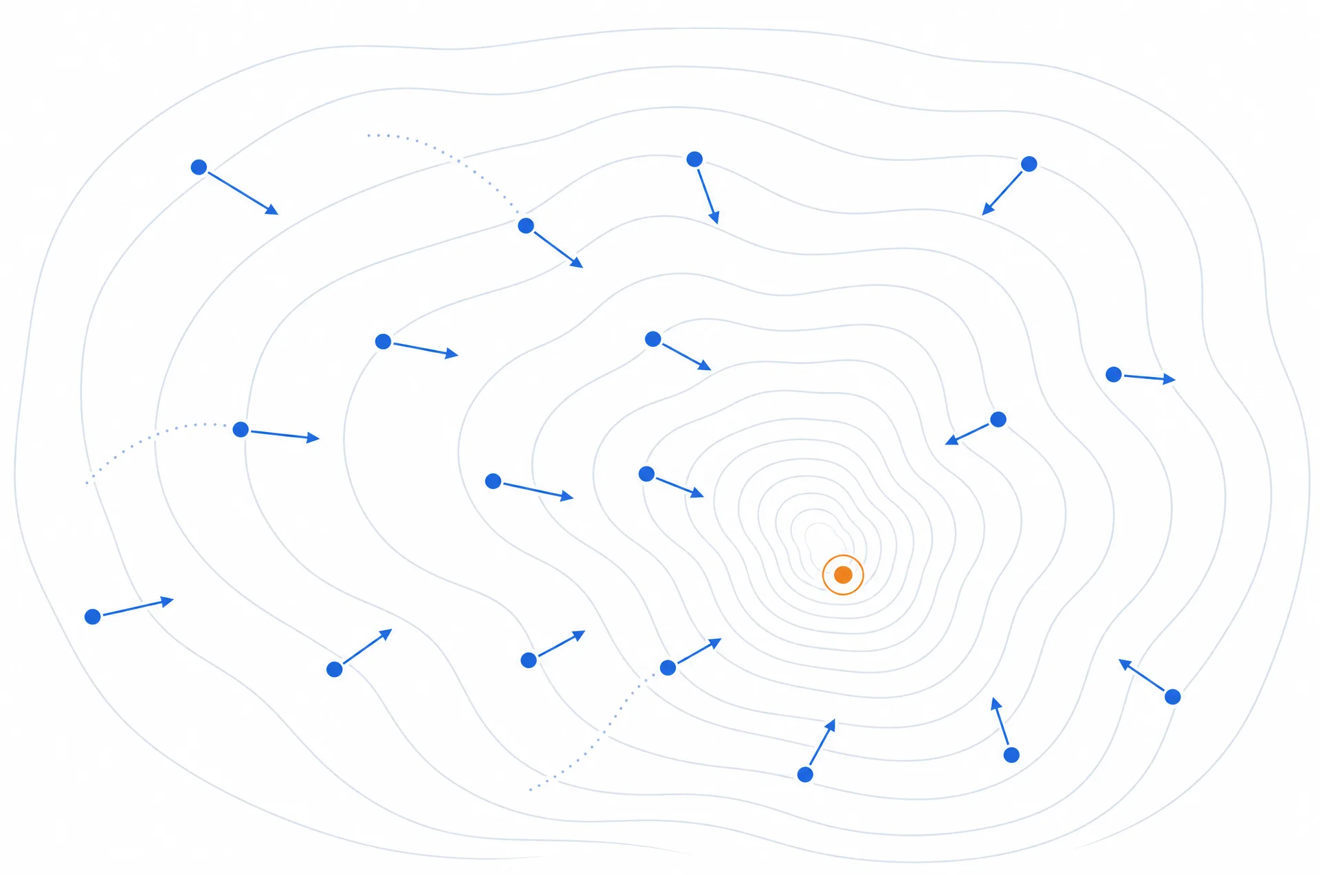
The illustration explains the search concept. It is not a plot from a run of the supplied code.

These repeated updates help the swarm explore promising regions. The result depends on the objective, bounds, parameters, and random choices. PSO does not guarantee a globally optimal solution.

The model taught in the course

Each particle $i$ has a position $x_i^t$ and a velocity $v_i^t$ at iteration $t$. It also remembers its personal best $p_i^t$, the best position it has visited. The swarm shares a global best $g^t$, the best position found by any particle. The course writes the standard update for each component $j$ of the vectors:

Here $w$ is the inertia coefficient, $c_1$ and $c_2$ are the acceleration coefficients, and $r_1$ and $r_2$ are random numbers drawn uniformly from $[0, 1]$. The three terms are the inertia term, the cognitive component and the social component. The PSO code post explains the math in more detail, with inertia weight damping and the constriction coefficients.

Parts of the course

Play playlistLoads from YouTube

The three parts are embedded above as a playlist, and each one is also linked on YouTube below.

Part 1/3: Theoretical Foundations

Length 22:11. Watch part 1 on YouTube (opens in a new tab).

• Origin of PSO (from 1:24). Kennedy and Eberhart were building a model of the social behavior of bird flocks and fish schools, and found that the model could solve optimization problems.
• A simple example (from 2:30). Two friends, Alice and Bob, search for the deepest point of a one-dimensional lake from their boats. They tell each other the depth they measure, and the one in the shallower place moves a step toward the other. Repeating this, they meet at the deepest point. The example shows the two principles behind PSO: communication and learning which location is better.
• Swarm intelligence (from 6:24). Simple agents, such as birds, ants or fish, reach together a level of intelligence that no single member could reach alone.
• Particles (from 7:43). Each particle has a position in the search space and a velocity of the same size. It also has a memory of its personal best, and the swarm has a common global best.
• The geometric picture (from 11:44). The new velocity combines three vectors: the old velocity, the vector toward the personal best, and the vector toward the global best. The particle then moves by this new velocity.
• The update equations (from 14:19). First in a simple vector form, then in the standard component-wise form with the random numbers $r_1$ and $r_2$ (from 17:05).
• The terms of the equations (from 19:43). The inertia term was not in the original 1995 version. It was added in 1998 by Shi and Eberhart. The other two terms are the cognitive and social components.

Part 2/3: Implementation in MATLAB

Length 39:12. Watch part 2 on YouTube (opens in a new tab).

• The test problem (from 0:04). The sphere function, $f(x) = \sum_{i=1}^{n} x_i^2$, whose minimum is at the origin. It is written as Sphere.m, so that the video can focus on PSO itself.
• Five sections of the code (from 2:15). Problem definition, parameters, initialization, main loop and results. The video notes that the other metaheuristics on Yarpiz share these sections.
• Problem definition (from 3:34). The cost function as a function handle, five decision variables stored as a row vector, and bounds of $-10$ and $10$.
• Parameters (from 8:40). The maximum number of iterations, the swarm size, and $w = 1$, $c_1 = 2$ and $c_2 = 2$.
• Initialization (from 11:01). A particle template is built as a MATLAB structure with the fields Position, Velocity, Cost and Best. The video explains repmat with a small matrix and uses it to create the swarm. Each particle gets a random position from unifrnd, a zero velocity and its cost, and its personal best starts at its first position.
• Global best (from 21:07). It starts with a cost of infinity, the worst value for a minimization problem, so the first particle compared with it always wins. An array BestCosts stores the best cost of every iteration.
• Main loop (from 26:13). Two nested loops over the iterations and the particles: update the velocity with element-wise products, update the position, evaluate the cost, then update the personal best and the global best. The best cost is displayed in each iteration with disp and num2str.
• Inertia weight damping (from 34:57). The first results are poor, so a damping ratio wdamp = 0.99 is added, and $w$ is multiplied by it in each iteration. The number of iterations is then raised to 1000.
• Results (from 36:04). The convergence plot is drawn with plot, then with semilogy, which shows the progress toward the origin much more clearly.

The video ends by noting that this code is for teaching. A professional application would need further changes.

Part 3/3: Improvements

Length 20:13. Watch part 3 on YouTube (opens in a new tab).

• A reusable function (from 0:04). The script becomes a function, out = PSO(problem, params). The structure problem holds the cost function, the number of variables and the bounds. The structure params holds the parameters, plus a flag ShowIterInfo that turns the iteration display on or off. The calling script becomes pso1.m.
• Position bounds (from 8:57). With a lower bound of 3, the search space no longer contains the origin, but the swarm still converges to the origin. The fix clips each position to the bounds with max and min after every move.
• Velocity limits (from 11:39). The velocity is clipped to $[-v_{\max}, v_{\max}]$, with $v_{\max} = 0.2\,(\text{VarMax} - \text{VarMin})$.
• Constriction coefficients (from 12:57). The configuration of Clerc and Kennedy (2002) is introduced and used in a second script, pso2.m, with no damping of $w$.
• Final test (from 18:15). pso2.m solves a 10-dimensional sphere problem.

The constriction coefficients, as computed in the video, are

with $w = \chi$, $c_1 = \chi\varphi_1$ and $c_2 = \chi\varphi_2$. The common choice is $\kappa = 1$ and $\varphi_1 = \varphi_2 = 2.05$, which gives $\chi \approx 0.7298$ and $c_1 = c_2 \approx 1.49$. In pso2.m this reads:

% Constriction Coefficients
kappa = 1;
phi1 = 2.05;
phi2 = 2.05;
phi = phi1 + phi2;
chi = 2*kappa/abs(2-phi-sqrt(phi^2-4*phi));

Course files

The project files and lecture notes are also available to download. The project files contain the scripts built in the videos: Sphere.m, the function PSO.m, and the two calling scripts pso1.m (the standard parameters with damping) and pso2.m (the constriction coefficients). Both scripts use 50 particles and 1000 iterations. PSO.m returns a structure with the final swarm (pop), the best solution (BestSol) and the best cost of each iteration (BestCosts).

Check the result

Follow the parts in order and run the Sphere example before replacing the objective. Part 2 introduces the search loop, while part 3 adds the bounds and velocity handling needed by the final version. Reproduce the bounded example and confirm that the returned position satisfies the bounds. If the origin is outside the search space, a cost near zero is not a valid target for that constrained problem.

Requirements

• Basic programming knowledge. Familiarity with MATLAB helps, and learners who know another language can translate the code easily.
• MATLAB, to follow the hands-on parts. The code creates random positions with unifrnd, which comes from the Statistics and Machine Learning Toolbox, so it probably needs that toolbox.

The course suits students and professionals who work on optimization problems, and anyone interested in computational intelligence.