Shuffled Complex Evolution in MATLAB

Shuffled Complex Evolution (SCE-UA) is a metaheuristic for global optimization, proposed by Duan, Sorooshian and Gupta in 1992 (paper (opens in a new tab)). The abbreviation SCE is used for other methods in science, so “UA” was added because the creators were members of the University of Arizona. The method was first developed to calibrate conceptual rainfall and runoff models in hydrology.

How SCE-UA works

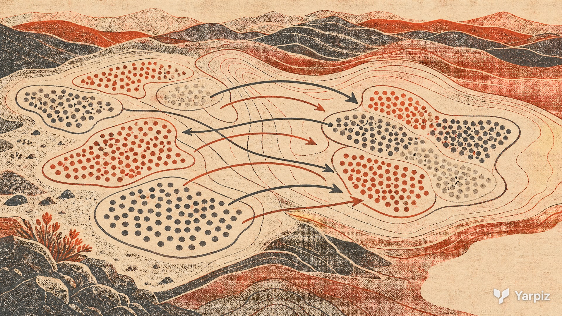
SCE-UA divides the population into sub-populations called complexes. At every iteration, an internal optimization mechanism called Competitive Complex Evolution (CCE) evolves each complex. After a CCE cycle on all complexes, they are combined to recreate the main population. The population is then partitioned again into new complexes, which shuffles the population and the complexes.

The Shuffled Frog Leaping Algorithm is a closely related metaheuristic and shares many properties with SCE-UA.

Forming the complexes

All members are sorted from best to worst and dealt to the complexes in turn: member 1 goes to complex 1, member 2 to complex 2, and so on. In this way, every complex holds both good and poor solutions.

Competitive Complex Evolution

CCE works like a few steps of the Nelder-Mead simplex method on a small random subset of the complex. In each CCE step:

1. Choose $q$ parents from the complex at random, with a higher probability for better members. For a complex of size $m$ sorted from best ($i = 1$) to worst, the code uses the probability $p_i = 2(m + 1 - i)/(m(m + 1))$.
2. Sort the parents, and compute the centroid $g$ of all parents except the worst one, $x_w$.
3. Reflection. Try $x_r = 2g - x_w$. If $x_r$ is outside the bounds, a random point in the smallest box that contains the complex is used instead. If $x_r$ is better than $x_w$, it replaces $x_w$.
4. Contraction. Otherwise, try $x_c = (g + x_w)/2$. If it is better, it replaces $x_w$.
5. Random point. Otherwise, replace $x_w$ with a random point in the smallest box that contains the complex.

The new parents go back into the complex, and the step repeats.

MATLAB implementation

This post shares an open-source, structured MATLAB implementation of SCE-UA. If you know MATLAB, you should find the code easy to use in your research projects.

The SCE-UA folder holds these files:

• sce.m: the main script, with the problem definition, the parameters and the main loop.
• RunCCE.m: one CCE run on a complex.
• Sphere.m: the sample cost function, $f(x) = \sum_{i=1}^{n} x_i^2$.
• SortPopulation.m, RandSample.m and IsInRange.m: helpers for sorting, weighted random selection and the bound check.
• main.m: a one line entry point that runs sce.m.

To run the code, open the SCE-UA folder in MATLAB and run main.m. The program prints the best cost in every iteration and plots the best cost against the iteration on a logarithmic scale. The code uses unifrnd and randsample, functions of the Statistics and Machine Learning Toolbox, so it probably needs that toolbox.

Parameters in the code

The complex size is at least nVar+1, the number of points of a simplex in nVar dimensions. To solve your own problem, write a cost function that takes a row vector and returns a number, and set CostFunction, nVar, VarMin and VarMax at the top of sce.m.

Check the result

The supplied Sphere problem has its minimum at the origin with cost 0. Inspect the best point as well as the cost curve, and compare repeated runs. Review complex size and the number of parents together when changing the dimension, since the local step builds a centroid from the selected parents. An outer iteration includes several local evaluations in each complex, so use evaluation counts for fair comparisons with other optimizers.

Mostapha Kalami Heris, Shuffled Complex Evolution in MATLAB (YPEA110), Yarpiz, 2015. https://yarpiz.com/shuffled-complex-evolution-ypea110

@misc{yarpiz-ypea110,
  author = {{Mostapha Kalami Heris}},
  title = {{Shuffled Complex Evolution in MATLAB}},
  howpublished = {Yarpiz},
  year = {2015},
  note = {Code YPEA110},
  url = {https://yarpiz.com/shuffled-complex-evolution-ypea110}
}