Interpolation and Curve Fitting in MATLAB: Video Tutorial

This video tutorial reviews interpolation and curve fitting and implements them in MATLAB. It is part of the Numerical Computations in MATLAB course.

Interpolation and curve fitting

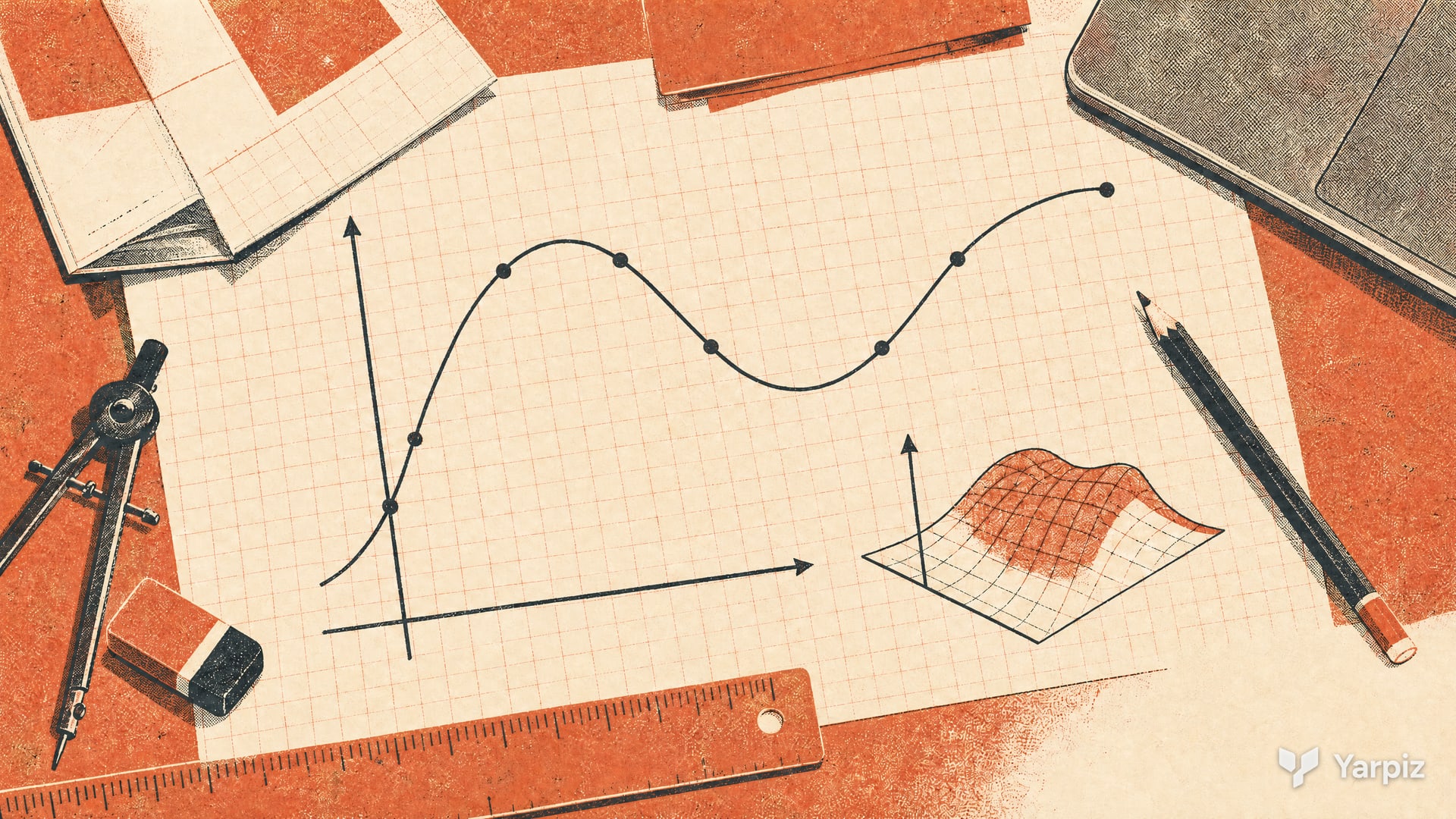
Both methods start from a set of data points $(x_i, y_i)$ and build a model that gives values between them. They differ in one important way:

• Interpolation builds a model that passes exactly through every data point, for example a straight line or a cubic piece between each pair of neighbors.
• Curve fitting chooses a simple model, such as a polynomial of degree $n$, that stays as close as possible to the points. With noisy data it does not pass through them. polyfit uses least squares: it picks the coefficients that minimize the sum of squared errors $\sum_i \left(y_i - p(x_i)\right)^2$.

The five videos move from one input variable to two and three, and from evenly spaced data to scattered points.

Watch online

The tutorial has five sections on YouTube. They are embedded below as a playlist.

Play playlistLoads from YouTube

Video sections

1. Polynomial fitting with polyfit

Polynomial fitting using polyfit (YouTube (opens in a new tab)). The function polyfit(x, y, n) takes the data and a degree $n$ and returns the coefficients of the polynomial. The video starts with three points of the known model $x^2 - 3x + 5$, and a fit of degree 2 returns exactly [1 -3 5].

It then draws 100 random points between $-1$ and $5$ and adds normally distributed noise. The fitted coefficients stay close to 1, $-3$ and 5, so polyfit recovers the model behind the noisy data. polyval evaluates the fitted polynomial for the plot. A degree of 1 gives the best straight line, and a degree of 3 adds a cubic term that the data does not need.

p = polyfit(x, y, 2);
yy = polyval(p, xx);

Finally, the second output S of polyfit is passed to polyval to get prediction error estimates delta at each point. The video plots yy + 2*delta and yy - 2*delta as an approximate prediction band. Its statistical interpretation depends on assumptions about the errors. It is not a guarantee that a fixed percentage of any data set lies inside the band.

2. Interpolation with interp1 to interpn

Interpolation using interp1 to interpn (YouTube (opens in a new tab)). These functions share one pattern: give the data points and the query points, and get the model values at the query points. interp1 handles one input, interp2 two inputs, interp3 three, and interpn any number.

The one dimensional example connects four data points. Linear interpolation draws a straight line between neighbors. Queries outside the data range require care: depending on the method and options, they may return NaN or an extrapolated value. Choose the behavior explicitly. The video compares linear, nearest, next, previous, pchip, cubic, makima and spline. Available methods differ between functions and MATLAB releases. In its higher dimensional examples, the video uses linear, nearest, cubic and spline.

The two dimensional example samples the peaks function on an 11 by 11 grid from $-5$ to $5$. interp2 then evaluates it on a grid with a spacing of 0.5 (441 points), and the cubic and spline methods give smoother surfaces than linear.

3. Interpolation with interpft

Interpolation using interpft (YouTube (opens in a new tab)). This function uses the Fourier transform. It moves the data to the frequency domain, interpolates there, and returns to the original domain with the inverse transform. This works well for data with a periodic pattern.

The example takes 30 evenly spaced samples of $f(x) = \sin(2x)\cos(x)$ up to $x = 4\pi$, and asks interpft(y, n) for 100 and then 300 points. interpft returns only the new values, so the video builds the matching $x$ values from the sample spacing and trims the output to the same length. At the end, these steps become a small helper function, myinterpft.

4. Interpolation with cubic splines

Interpolation using cubic splines (YouTube (opens in a new tab)). The spline function gives the same result as the spline method of interp1, and it can also return the piecewise polynomial form of the model.

The first example fits a smooth curve through a few points and shows how the curve changes as points are added. The second example builds a smooth path in the plane. A source at $(0, 0)$, a destination at $(5, 5)$ and a few random handle points are joined, and $x$ and $y$ are each interpolated as functions of a parameter $t$ from 0 to 1:

t  = linspace(0, 1, numel(x));
tt = linspace(0, 1, 100);
xx = spline(t, x, tt);
yy = spline(t, y, tt);

The video explains that this idea is useful in mobile robot path planning and optimal control. A metaheuristic such as a genetic algorithm can then search among the handle points for the best smooth path. A related example is Optimal Robot Path Planning Using PSO in MATLAB.

5. Scattered data with griddata

Interpolation using griddata in 2D and 3D spaces (YouTube (opens in a new tab)). griddata works like interp2 and interp3, but the data points do not need to lie on a grid. Its methods are linear, nearest, natural (natural neighbor interpolation, based on triangulation), cubic and v4.

The example draws 100 random points with $x$ and $y$ between $-3$ and $3$, computes a function value at each point and shows them with plot3. griddata then evaluates the model on a regular grid with a spacing of 0.25 (625 points), and mesh shows the surface. The cubic method gives a smooth result. The video also mentions griddatan for data with more input variables.

Choosing a method

• Noisy data and a simple model: polyfit and polyval.
• Data on a grid: interp1, interp2, interp3 or interpn.
• Periodic, evenly spaced data: interpft.
• A smooth curve or path through given points: spline.
• Scattered data in two or three dimensions: griddata.

Check the model

Plot the original samples together with the fitted or interpolated curve. High degree polynomials and smooth splines can oscillate between samples, so a smooth result is not automatically a good model. Keep extrapolated values separate from values inside the sampled region. For noisy data, compare fits using points that were not used to estimate the coefficients.