Numerical Solution of Differential Equations in MATLAB: Video Tutorial

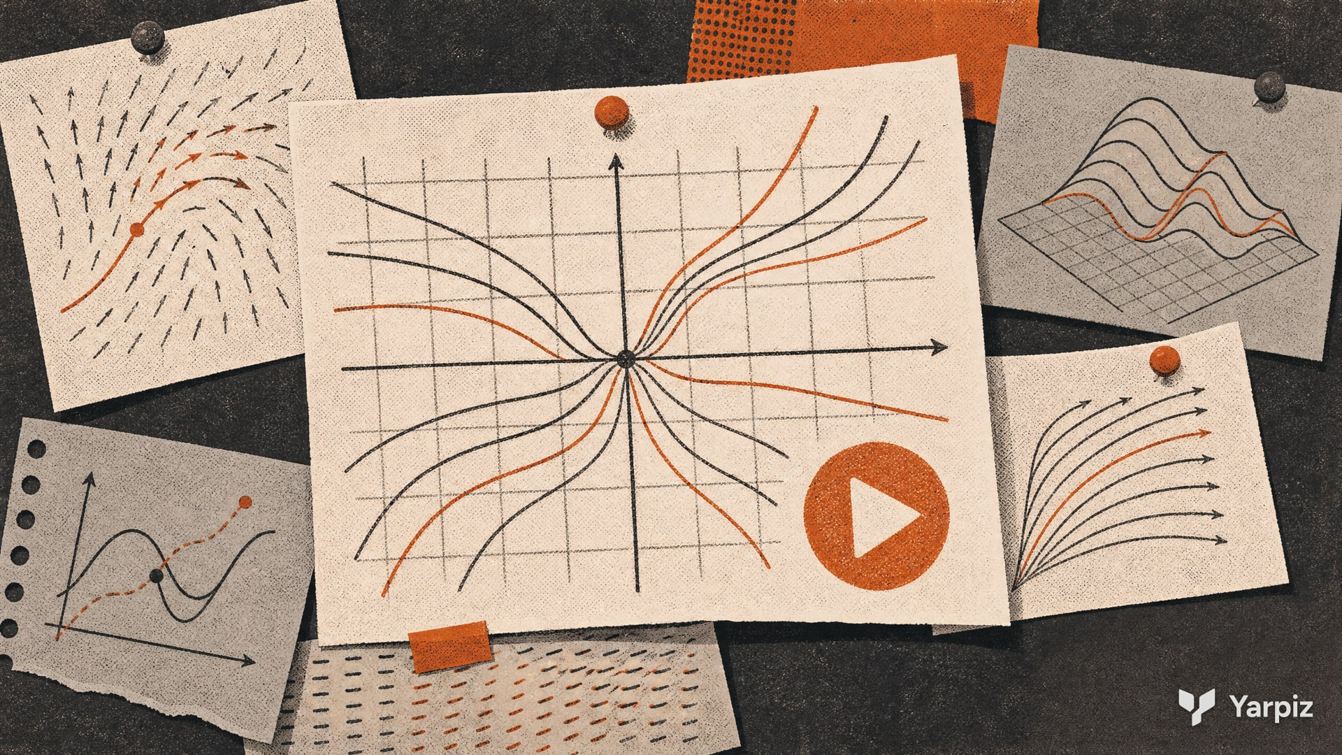
This video tutorial reviews the numerical solution of differential equations and implements it in MATLAB. It is part of the Numerical Computations course.

Three kinds of problems

The ODE and BVP examples use systems of first order equations:

Here $t$ is the independent variable and $y$ can be a vector. An equation of higher order is first rewritten as a first order system. For example, $x'' = g(x, x')$ becomes two equations with $y_1 = x$ and $y_2 = x'$:

The three videos then treat three kinds of problems:

• Initial value problems (ODEs): the state is known at the start time, $y(t_0) = y_0$.
• Boundary value problems (BVPs): conditions are given at both ends of an interval $[a, b]$.
• Delay differential equations (DDEs): the rate of change also depends on past states, such as $y(t - \tau)$.

Watch online

The three sections are available on YouTube and embedded below as a playlist.

Play playlistLoads from YouTube

What each video covers

Section 1: Ordinary differential equations

Solving Ordinary Differential Equations (YouTube (opens in a new tab)). The video first sorts the MATLAB ODE solvers into two groups:

• Nonstiff solvers: ode45, ode23 and ode113. Try ode45 first, as it solves most problems well. ode23 can be better with crude tolerances or moderate stiffness, and ode113 with strict tolerances or a model that is expensive to evaluate.
• Stiff solvers: ode15s, ode23s, ode23t and ode23tb. The video compares these methods on its examples. Their relative speed and accuracy depend on the equations, tolerances and solver settings, so there is no fixed ranking for every model.

The first example is $y' = -y + 2t$ with $y(0) = 1$ on $[0, 2]$. A solver call needs the function, the time span and the initial condition:

f = @(t, y) -y + 2*t;
[t, y] = ode45(f, [0 2], 1);
plot(t, y)

The video changes the initial condition and compares ode45 with ode23 (which gives a less smooth result) and ode113.

The second example is the van der Pol oscillator:

It becomes a first order system with $y_1 = x$ and $y_2 = x'$. The model is written as a function with $\mu$ as an extra parameter, and an anonymous function passes the value of $\mu$ to it. A phase plane plot of $y_2$ against $y_1$ shows the limit cycle. With $\mu = 0$ the system is a pure oscillator and the phase plot is a circle. As $\mu$ grows the model becomes stiff, ode45 slows down, and ode15s solves it faster.

The third example is the Lorenz system, a chaotic model with three states:

With $\sigma = 10$, $\rho = 28$, $\beta = 8/3$ and the initial state $(1, 0, 0)$, ode45 and plot3 show the Lorenz attractor.

Section 2: Boundary value problems

Solving Boundary Value Problems (YouTube (opens in a new tab)). MATLAB solves BVPs with bvp4c and bvp5c, which use collocation methods of fourth and fifth order. They are called in the same way. Besides the ODE function, you write a function for the boundary conditions in the form $g\big(y(a), y(b)\big) = 0$, and you give an initial guess built with bvpinit.

The first example is

which becomes $y_1' = y_2$ and $y_2' = -y_1$. The boundary condition function returns [ya(1) - 1; yb(1)].

f  = @(x, y) [y(2); -y(1)];
bc = @(ya, yb) [ya(1) - 1; yb(1)];
solinit = bvpinit(linspace(0, pi/2, 100), [1 0]);
sol = bvp4c(f, bc, solinit);
plot(sol.x, sol.y(1, :))

The solution sol has the fields x, y and yp. Changing a boundary condition changes the mathematical problem. Depending on the equations and the new conditions, a BVP may have one solution, several solutions or no solution, and the initial guess can affect which solution a numerical solver finds.

The second example has a condition on the derivative: the equation $y'' - 2y' + 2y = 0$ on $[0, 2]$ with $y(0) = 1$ and $y'(2) = -1$. Here the second condition uses the second state, yb(2) + 1.

Section 3: Delay differential equations

Solving Delayed Differential Equations (YouTube (opens in a new tab)). A DDE also needs a history: the solution for all times before the start. MATLAB has three solvers:

• dde23 for constant delays.
• ddesd for delays that depend on time or on the state.
• ddensd for neutral equations, where the derivative $y'$ also appears with a delay.

The video solves four examples:

1. The scalar equation $y'(t) = 2y(t) - y(t - 1) - 1$ with the history $y = 1$, solved with dde23 on $[0, 5]$. The function deval evaluates the solution at chosen times. The video also tries other histories, such as $\cos t$.
2. A system of three equations with two constant delays, 1 and 0.5, and the history $(1, 0, -1)$. Each column of the lag matrix holds the states at one delay.
3. A system with a state dependent delay, solved with ddesd:
   $$y_1'(t) = y_2(t), \qquad y_2'(t) = -y_2\big(d(t)\big)\, y_2(t)^2\, e^{1 - y_2(t)}, \qquad d(t) = e^{1 - y_2(t)}$$
   The video compares the result with $y_1 = \ln t$ and $y_2 = 1/t$ and starts at 0.1 rather than 0. The displayed comparison functions are not defined at $t = 0$. A DDE history must also be defined at every past time the solver requests. Check the delay arguments and the history domain when adapting this example.
4. A neutral equation, solved with ddensd:
   $$y'(t) = 1 + y(t) - 2\,y(t/2)^2 - y'(t - \pi)$$
   Its exact solution and history is $y = \cos t$. The video plots the numerical and exact solutions together, and the error is small.

Applications

• Simulating dynamic systems such as oscillators, circuits and chaotic models.
• Boundary value problems in mechanics and heat transfer, such as the shape of a beam or a temperature profile.
• Models with delays, for example in control systems and population dynamics.

The Runge-Kutta video tutorial shows how a classic ODE method works inside, in Python and MATLAB.

Check the solution

Compare results at tighter tolerances and inspect initial or boundary residuals. A convincing plot alone does not establish accuracy. For a delay model, verify that the history matches the intended past states and uses the same state ordering as the derivative function. In chaotic systems such as Lorenz, trajectories can separate over time even when both runs are numerically reasonable.