Parallel Machine Scheduling using Simulated Annealing

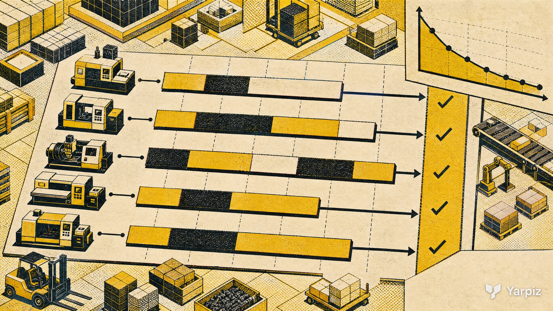
This package implements Parallel Machine Scheduling in MATLAB and solves it with Simulated Annealing (SA). The goal is to assign jobs to machines and order them so that the makespan (Cmax, the completion time of the last machine) is as small as possible.

Parallel machine scheduling is a classic problem in production planning. Several machines work at the same time, and each job needs one machine. The version in this code is one of the harder ones: the machines are unrelated (the processing time of a job depends on the machine), and the setup time between two jobs depends on their order. Even the simplest version with two identical machines is NP-hard, so metaheuristics such as SA are a common choice.

The problem

There are $I$ jobs and $J$ machines. The data are:

• $p_{ij}$: the processing time of job $i$ on machine $j$.
• $s_{kij}$: the setup time on machine $j$ when job $i$ follows job $k$.

A schedule assigns each job to exactly one machine and gives the order of the jobs on each machine. A machine does one job at a time, without breaks. If job $i$ follows job $k$ on machine $j$, it starts when job $k$ finishes plus the setup time:

The first job on a machine starts at time 0 with no setup. If $C_j$ is the finish time of the last job on machine $j$, the objective is the makespan:

In the standard three field notation, this is the problem $R \mid s_{kij} \mid C_{\max}$.

The sample model in CreateModel.m has 20 jobs and 4 machines. The processing times are between 10 and 60, and the setup times are between 2 and 8.

How a solution is encoded

A solution is a permutation of the numbers 1 to $I + J - 1$ (23 numbers in the sample). The numbers 1 to $I$ are jobs, and the numbers above $I$ are separators. Reading from left to right, the jobs before the first separator go to machine 1 in that order, the jobs between the first and second separators go to machine 2, and so on. A machine may get no jobs.

ParseSolution.m decodes the permutation this way and then simulates the schedule with the formulas above. It returns the start and finish time of every job, the completion time of each machine and the makespan. MyCost.m returns the makespan as the cost.

How Simulated Annealing searches

SA keeps one current solution. At each temperature it tries MaxIt2 neighbors. CreateNeighbor.m makes a neighbor with one of three moves, chosen with equal probability:

• Swap: exchange two entries. This can move two jobs between machines or change their order.
• Reversion: reverse the order of a part of the permutation.
• Insertion: take one entry and put it in another position.

Because separators are also entries, each move can change the assignment of jobs to machines as well as the order on a machine.

A better or equal neighbor is always accepted. A worse one is accepted with probability $\exp(-\Delta / T)$, where $\Delta$ is the increase in makespan and $T$ is the temperature. After each outer iteration the temperature is multiplied by alpha. For a full explanation of the method, see the Simulated Annealing post.

What is in the package

• CreateModel.m defines a sample problem with 20 jobs and 4 machines. It holds a matrix of processing times and a set of setup times for each machine.
• CreateRandomSolution.m creates a random initial solution.
• CreateNeighbor.m creates a neighbor of a solution by swap, reversion or insertion.
• ParseSolution.m converts a solution into job sequences for the machines and simulates the schedule to find the makespan.
• MyCost.m is the cost function. It returns the makespan.
• PlotSolution.m plots a solution.
• sa.m is the main script. It sets the SA parameters (500 iterations, 25 inner iterations, initial temperature 10, damping rate 0.97) and runs the algorithm.

How to use

Open sa.m in MATLAB and run it. To solve your own problem, replace the data in CreateModel.m.

The program prints the best makespan in every iteration. PlotSolution.m draws the best schedule as a Gantt chart, with one row per machine, one colored bar per job and a red line at $C_{\max}$. At the end, a second figure shows the best cost against the iteration. CreateNeighbor.m calls randsample, so the code probably needs the Statistics and Machine Learning Toolbox.

Parameters in the code

Check the result

Verify that every job appears once, machine processing times come from the correct column, and each setup time uses the correct ordered pair of jobs. Recompute the makespan from the decoded finish times. The example omits release dates, due dates, breakdowns, and other operational constraints, so those need explicit model changes if they matter to your schedule. Compare repeated runs on the same data rather than treating a single Gantt chart as evidence of optimality.

Applications

Problems of this type appear in many workshops and service systems:

• Production lines with several machines that can do the same operations at different speeds.
• Printing, painting and chemical plants, where cleaning or changeover time depends on the previous job.
• Assigning tasks to processors in computing.
• Scheduling operating rooms or service counters.

Related posts

• Simulated Annealing in MATLAB
• Capacitated Vehicle Routing Problem using Simulated Annealing, which uses the same separator encoding and the same neighbor moves.
• Bin Packing Problem using GA, PSO, FA and IWO

Mostapha Kalami Heris, Parallel Machine Scheduling using Simulated Annealing (YPAP107), Yarpiz, 2015. https://yarpiz.com/parallel-machine-scheduling-ypap107

@misc{yarpiz-ypap107,
  author = {{Mostapha Kalami Heris}},
  title = {{Parallel Machine Scheduling using Simulated Annealing}},
  howpublished = {Yarpiz},
  year = {2015},
  note = {Code YPAP107},
  url = {https://yarpiz.com/parallel-machine-scheduling-ypap107}
}