Capacitated Vehicle Routing Problem (VRP) Using Simulated Annealing in MATLAB

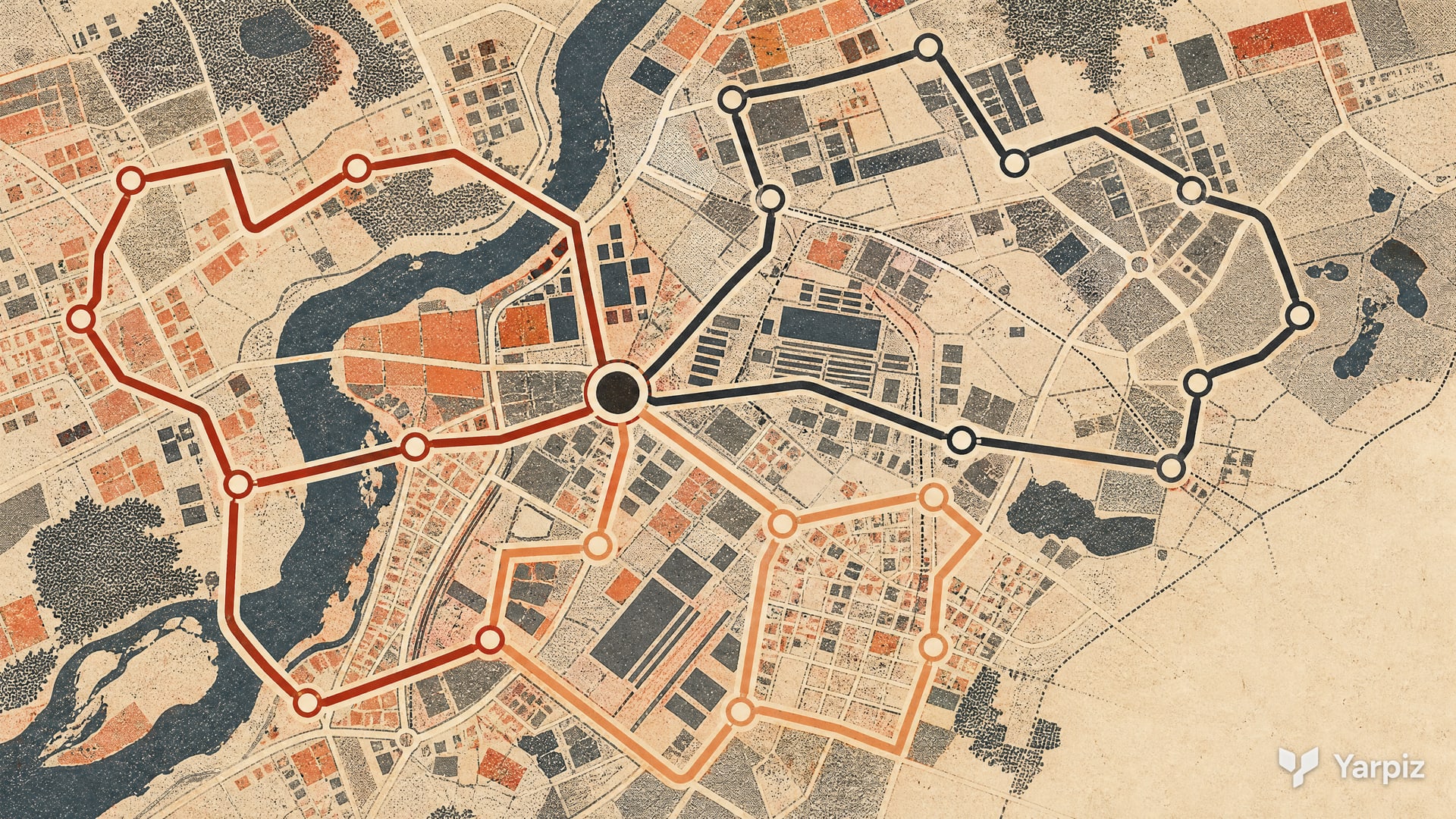
This package solves the Capacitated Vehicle Routing Problem (VRP) in MATLAB with Simulated Annealing (SA). Several vehicles with limited capacity must serve customers that have known demands and locations.

The Vehicle Routing Problem was introduced by Dantzig and Ramser in 1959 as the “truck dispatching problem”. It generalizes the Traveling Salesman Problem (TSP) to several vehicles, so it is NP-hard. Exact methods can solve small and medium instances, but metaheuristics such as SA, Tabu Search and Genetic Algorithms are widely used for larger ones.

The problem

There is one depot and $I$ customers. Customer $i$ has a demand $r_i$, and vehicle $j$ has a capacity $c_j$. The distance between customers $i$ and $k$ is $d_{ik}$, and the distance from the depot to customer $i$ is $d_{0i}$.

Each vehicle $j$ drives one route $L_j$: it leaves the depot, visits its customers in order and returns to the depot. A solution must satisfy these rules:

• Every customer is visited exactly once, by exactly one vehicle.
• The total demand on a route does not exceed the capacity of its vehicle: $\sum_{i \in L_j} r_i \le c_j$.
• A vehicle may stay unused.

The classic CVRP minimizes the total distance $\sum_j D_j$, where $D_j$ is the length of route $j$. In this code, the vehicles may have different capacities, and the objective mixes the total distance with the length of the longest route.

The cost function

ParseSolution.m computes the length $D_j$ of each route, the load of each vehicle and the capacity violation $CV_j = \max(\text{load}_j / c_j - 1, \; 0)$. MyCost.m then combines them:

Here $\overline{CV}$ is the mean violation over the vehicles and $\beta = 5$. The weight $\eta$ is stored in the model, and sa.m sets it to 0.1, so the longest route has most of the weight. This favors reducing the longest route while still accounting for total distance. With $\eta = 1$ the cost would be the classic total distance. A solution with $\overline{CV} = 0$ is feasible.

How a solution is encoded

A solution is a permutation of the numbers 1 to $I + J - 1$, where $J$ is the number of vehicles. The numbers 1 to $I$ are customers, and the numbers above $I$ are separators. Reading from left to right, the customers before the first separator form the route of vehicle 1 in that order, the customers between the first and second separators form the route of vehicle 2, and so on.

CreateNeighbor.m changes a solution with one of three moves, chosen with equal probability: swap two entries, reverse a part of the permutation, or move one entry to another position. Because the separators are entries too, a move can change the order within a route or move customers between vehicles.

SA accepts a better neighbor at once and a worse one with probability $\exp(-\Delta / T)$. For a full explanation of the method, see the Simulated Annealing post.

What is in the package

• sa.m: the Simulated Annealing algorithm. main.m starts it.
• CreateNeighbor.m: creates a neighbor solution by a random swap, reversion or insertion move.
• MyCost.m and ParseSolution.m: decode a solution and compute its cost. The cost combines total distance, maximum route distance and a penalty term for capacity violations.
• CreateRandomModel.m and CreateRandomSolution.m: generate random problem data and random starting solutions.
• SelectModel.m and the vrp_*.mat files: ready-made models with different numbers of customers and vehicles (for example 8 customers with 3 vehicles, up to 70 customers with 8 vehicles).
• VRP Model Creation/CreateAndSaveModels.m: creates and saves new models.
• PlotSolution.m: plots the routes.

The ten saved models are vrp_8x3, vrp_10x3, vrp_14x4, vrp_20x4, vrp_25x5, vrp_30x5, vrp_40x6, vrp_50x7, vrp_60x7 and vrp_70x8, where the first number is the number of customers and the second the number of vehicles. In CreateRandomModel.m, customers are placed at random on a 200 by 100 area, the depot is near the center, demands are between 10 and 25, and each vehicle capacity is chosen at random between the total demand divided by the number of vehicles and 1.25 times that value.

How to run

Run main.m.

A file dialog opens. Choose one of the vrp_*.mat files. The program prints the best cost in every iteration and adds a * when the best solution is feasible. It draws the routes of the best solution, each vehicle in its own color, with the depot as a yellow square. At the end it plots the best cost against the iteration. CreateNeighbor.m calls randsample, so the code probably needs the Statistics and Machine Learning Toolbox.

Parameters in the code

Check the result

Confirm that every customer appears exactly once, every route starts and ends at the depot, and every vehicle load is within its own capacity. Report total distance and longest-route distance separately from the penalized score. Setting eta to 1 gives the total-distance objective only for a feasible solution, since the capacity penalty still applies. Repeat runs on the same saved model and check feasibility even when the cost improves.

Applications

Vehicle routing is one of the most used models in logistics:

• Parcel and grocery delivery from a warehouse.
• Waste collection and street cleaning.
• School bus routing.
• Field service and maintenance visits.

Related posts

• Simulated Annealing in MATLAB
• Parallel Machine Scheduling using Simulated Annealing, which uses the same encoding and neighbor moves.
• Tabu Search in MATLAB, another local search method, applied to the TSP.

Mostapha Kalami Heris, Capacitated Vehicle Routing Problem (VRP) Using Simulated Annealing in MATLAB (YPAP108), Yarpiz, 2015. https://yarpiz.com/vehicle-routing-problem-ypap108

@misc{yarpiz-ypap108,
  author = {{Mostapha Kalami Heris}},
  title = {{Capacitated Vehicle Routing Problem (VRP) Using Simulated Annealing in MATLAB}},
  howpublished = {Yarpiz},
  year = {2015},
  note = {Code YPAP108},
  url = {https://yarpiz.com/vehicle-routing-problem-ypap108}
}