Runge-Kutta Method in Python and MATLAB: Video Tutorial
Build an RK4 solver in Python and MATLAB, simulate a predator-prey model and compare step sizes to understand accuracy and the limits of a fixed-step method.


On this page
This video tutorial explains the fourth order Runge-Kutta method (RK4) for the numerical solution of ordinary differential equations (ODEs). The method is then implemented from scratch in MATLAB and Python. As an example, the Lotka-Volterra model (also called the predator-prey model) is simulated with RK4 in both languages.
Mostapha Kalami Heris teaches the 35 minute 49 second video, which covers the formulas, a MATLAB solver and a matching Python implementation.
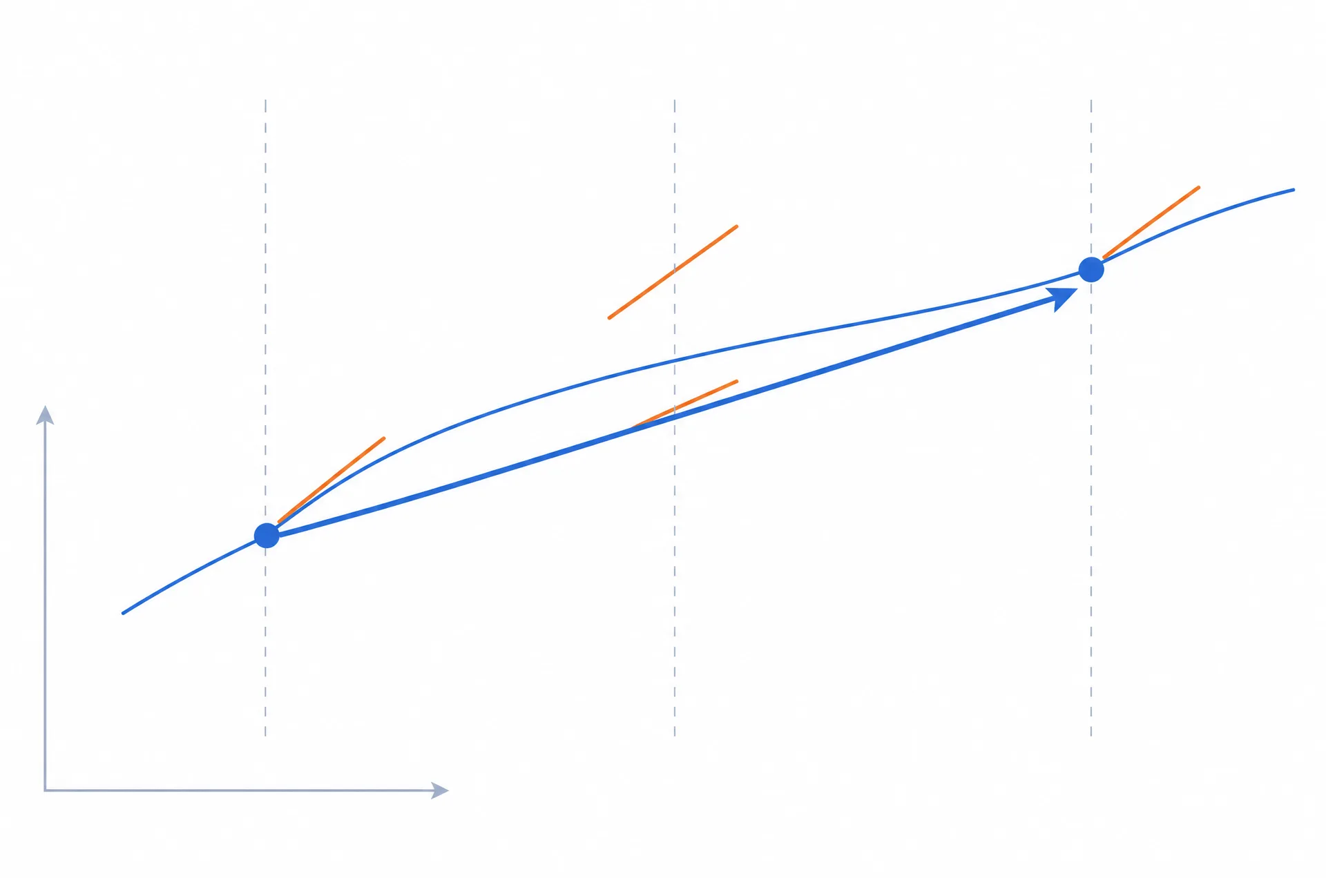
This conceptual sketch illustrates the four slope samples within one step. It is not output from the predator-prey simulation.
The problem: an initial value problem
An ODE describes how a quantity changes over time, for example the size of a population. The video writes the general problem in this form:
Here is the state. It does not have to be a single number. It can be a vector, so the same form covers a system of several coupled equations. When the equations are nonlinear, an exact solution is often hard or impossible to find, and a numerical method computes the solution step by step instead.
MATLAB and Python both have ready-made ODE solvers. The video still writes RK4 from scratch, for teaching purposes. Knowing the method line by line makes it possible to change it or to write other methods for other types of problems.
The RK4 method
Runge-Kutta methods are a family of methods for solving ODEs, named after Carl Runge and Martin Kutta. RK4 is the best known member of the family. It advances the solution from time to , where is the step size (the sample time). At each step it evaluates the function four times:
The new state is the old state plus a weighted average of these four increments:
The terms and sample the slope at the middle of the time step, at different estimated states. They get twice the weight of and . For a sufficiently smooth problem, the local error of a step started from the exact state is of order . Under the usual stability assumptions, the global error over a fixed time span is of order , which is why the method is called fourth order.
The example: the Lotka-Volterra model
The Lotka-Volterra equations describe the populations of two species, a prey and a predator :
Without predators, the prey grows at the rate . Meetings between the two species reduce the prey and help the predators grow. Without prey, the predators decline at the rate . The two equations are stacked into one state vector , so the system has the form . The model does not depend on time explicitly, so is accepted as an input but not used.
The video uses these values:
| Parameter | Value |
|---|---|
| 1.1 | |
| 0.4 | |
| 0.4 | |
| 0.1 | |
| Initial state |
What the video covers
Theory (from 00:07)
The video introduces the Runge-Kutta family, the RK4 formulas and the general problem . It then rewrites the Lotka-Volterra equations in this form and chooses the parameters and the initial state above (01:29 to 05:32).
MATLAB implementation (from 05:32)
- A model function returns the time derivative of the state. It takes the time and the state as inputs, so it fits the general form even though it ignores the time.
- An RK4 function takes the model , the initial state, the initial time, the final time and the step size (from 09:32). It builds the time vector, prepares a matrix with one column per time point, sets the first column to the initial state and then applies the four step formulas in a loop.
- A script then defines the problem and calls RK4 (from 16:22). The parameters are moved into a structure, and an anonymous function passes them to the model. The first run goes from to with a step of .
- The results are plotted (from 20:22): the prey and predator populations over time, with the time window extended to 50, and a phase plot of predators against prey. The phase plot is a closed loop, which shows that the populations repeat in cycles.
Python implementation (from 23:01)
The same program is written in Python with NumPy and Matplotlib. The parameters are kept in a dictionary, a lambda function passes them to the model, and the RK4 function builds the time vector with numpy.arange and fills a NumPy array in a loop. Python arrays start at index 0, so the indices change. The video ends with the same two plots and shows that the results are the same as in MATLAB.
Applications
ODEs appear whenever a model describes change over time: motion in mechanics, electric circuits, chemical reactions, population dynamics and the control of dynamic systems. A fixed-step RK4 implementation is useful for learning and for smooth, nonstiff problems where the step size is chosen carefully. It has no built-in error estimate or automatic step selection.
Check the step size
Run the model with the same parameters and final time, first with step and then with . Compare the states at matching times. Large changes suggest that the coarser run is not accurate enough. Population values should remain nonnegative in this model, so negative numerical values are a warning to inspect the implementation and step size. Stiff problems may need a different solver rather than only a smaller fixed step.
Who this tutorial is for
- Applied mathematics and science students
- Engineering students
- Software engineers and programmers interested in numerical computation
It helps to know the basics of differential equations and of programming in Python or MATLAB. The video explains each step of the code.
Watch online
The video tutorial is available on the Yarpiz YouTube channel.

How to cite
If you use this code or tutorial in your work, articles or publications, please cite it.
Mostapha Kalami Heris, Runge-Kutta Method in Python and MATLAB: Video Tutorial (YPTDEQ190515), Yarpiz, 2019. https://yarpiz.com/runge-kutta-rk4-in-python-and-matlab-yptdeq190515@misc{yarpiz-yptdeq190515,
author = {{Mostapha Kalami Heris}},
title = {{Runge-Kutta Method in Python and MATLAB: Video Tutorial}},
howpublished = {Yarpiz},
year = {2019},
note = {Code YPTDEQ190515},
url = {https://yarpiz.com/runge-kutta-rk4-in-python-and-matlab-yptdeq190515}
}Published Updated
Comments