Working with Polynomials in MATLAB: Video Tutorial
Work with MATLAB coefficient vectors to evaluate, fit, multiply, divide, differentiate and integrate polynomials. Check roots and division remainders.


On this page
This video tutorial shows how to work with polynomials in MATLAB. It reviews the functions that evaluate polynomials, find and use their roots, fit them to data, multiply and divide them, and compute their derivatives and integrals. To watch the full course, see Numerical Computations in MATLAB.
How MATLAB represents a polynomial
MATLAB stores the polynomial
as the row vector of its coefficients, from the highest power down to the constant term: [an an-1 ... a1 a0]. A missing power gets a zero. All the functions in this video use this form. The main example is
which is the vector [1 0 -2 5], because the term is absent.
Watch online
The video is available on YouTube and is embedded below.
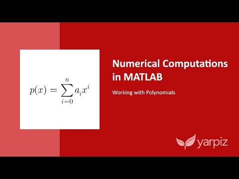
What the video covers
Working with Polynomials (YouTube (opens in a new tab)) introduces the functions one by one. Several of them come in pairs, where one function undoes the other. The times below mark where each topic starts.
Evaluating a polynomial with polyval (from 2:43)
polyval(p, x) evaluates the polynomial at one point or at a whole vector of points. For the example, and . Evaluated on many points, the plot shows one real root a little below .
p = [1 0 -2 5];
polyval(p, [0 1 2])   % 5  4  9
Roots and polynomials with roots and poly (from 5:22)
roots(p) returns the roots: one real root (about ) and a pair of complex conjugate roots. A polynomial of odd degree with real coefficients always has at least one real root. poly(r) does the opposite: it builds the polynomial from a list of roots.
The two are not complete inverses. The polynomial has the same roots as , and poly always returns a polynomial whose first coefficient is 1.
Fitting a polynomial with polyfit (from 8:01)
Four points of , at , are passed to polyfit with a degree of 3, and it returns [1 0 -2 5], the original polynomial. Lower degrees give the closest polynomial of that degree to the same data. The constant fit is , the mean of the four values. A loop fits degrees 0 to 3 and plots the four approximations together, with a legend made from DisplayName. Fitting noisy data is covered in the interpolation and curve fitting tutorial.
Multiplication and division with conv and deconv (from 13:31)
Multiplying two polynomials is the same as convolving their coefficient vectors. With :
q = [1 0 2];
r = conv(p, q)      % [1 0 0 5 -4 10]
deconv(r, p)        % returns q
deconv divides polynomials and can return both a quotient and a remainder. In this example the divisions are exact: deconv(r, p) returns and deconv(r, q) returns . A general division need not have a zero remainder.
Derivatives and integrals with polyder and polyint (from 16:17)
polyder returns the exact derivative. For the examples, , which is [3 0 -2], and .
polyint returns the integral. By default the constant of integration is 0, so polyint(p) gives . A second input sets the constant: polyint(q, -1) gives . Taking the derivative of an integral returns the original polynomial, while integrating a derivative loses the constant term unless you pass it back.
Summary of the functions
| Task | Function | Inverse |
|---|---|---|
| Evaluate | polyval |
|
| Roots | roots |
poly |
| Fit to data | polyfit |
|
| Multiply | conv |
deconv |
| Differentiate | polyder |
polyint |
Check the calculation
Keep zero coefficients for missing powers. Dropping one changes the polynomial rather than shortening its representation. Evaluate a polynomial at its computed roots to inspect the residuals, and reconstruct a division from the divisor, quotient and remainder. High degree polynomials and repeated or closely spaced roots can be sensitive to rounding, so avoid treating every displayed digit as accurate.
How to cite
If you use this code or tutorial in your work, articles or publications, please cite it.
Mostapha Kalami Heris, Working with Polynomials in MATLAB: Video Tutorial (YPTNM190520S16), Yarpiz, 2019. https://yarpiz.com/working-with-polynomials-video-tutorial-yptnm190520s16@misc{yarpiz-yptnm190520s16,
author = {{Mostapha Kalami Heris}},
title = {{Working with Polynomials in MATLAB: Video Tutorial}},
howpublished = {Yarpiz},
year = {2019},
note = {Code YPTNM190520S16},
url = {https://yarpiz.com/working-with-polynomials-video-tutorial-yptnm190520s16}
}Published Updated
Comments